Here’s the myth: Maple Grove is the affordable family suburb, and Saint Paul is the expensive urban core. In 2026, that story doesn’t hold up the way people expect. Both cities sit in the Minneapolis–Saint Paul metro, share the same regional price environment, and face identical utility and fuel costs. But the cost experience — where money goes, what flexibility you have, and how much friction daily life creates — differs sharply depending on household structure, commute tolerance, and whether you value predictability over space.
This isn’t about which city costs less overall. It’s about where cost pressure concentrates and which households feel it most. Maple Grove offers suburban space and a median home value of $379,800, but requires a car for nearly everything and clusters grocery and errands along commercial corridors. Saint Paul provides rail transit, broadly accessible daily errands, and stronger family infrastructure, but housing data for 2026 remains incomplete, making direct numeric comparison impossible. What we can compare: how the same income feels different depending on which costs dominate your household budget and how much time you spend managing logistics.
The decision between these two cities comes down to tradeoffs between housing entry costs, transportation dependence, and the daily friction of getting things done. Families, singles, and couples all face different exposures — and the right fit depends on which costs you can absorb and which you can’t.
Housing Costs
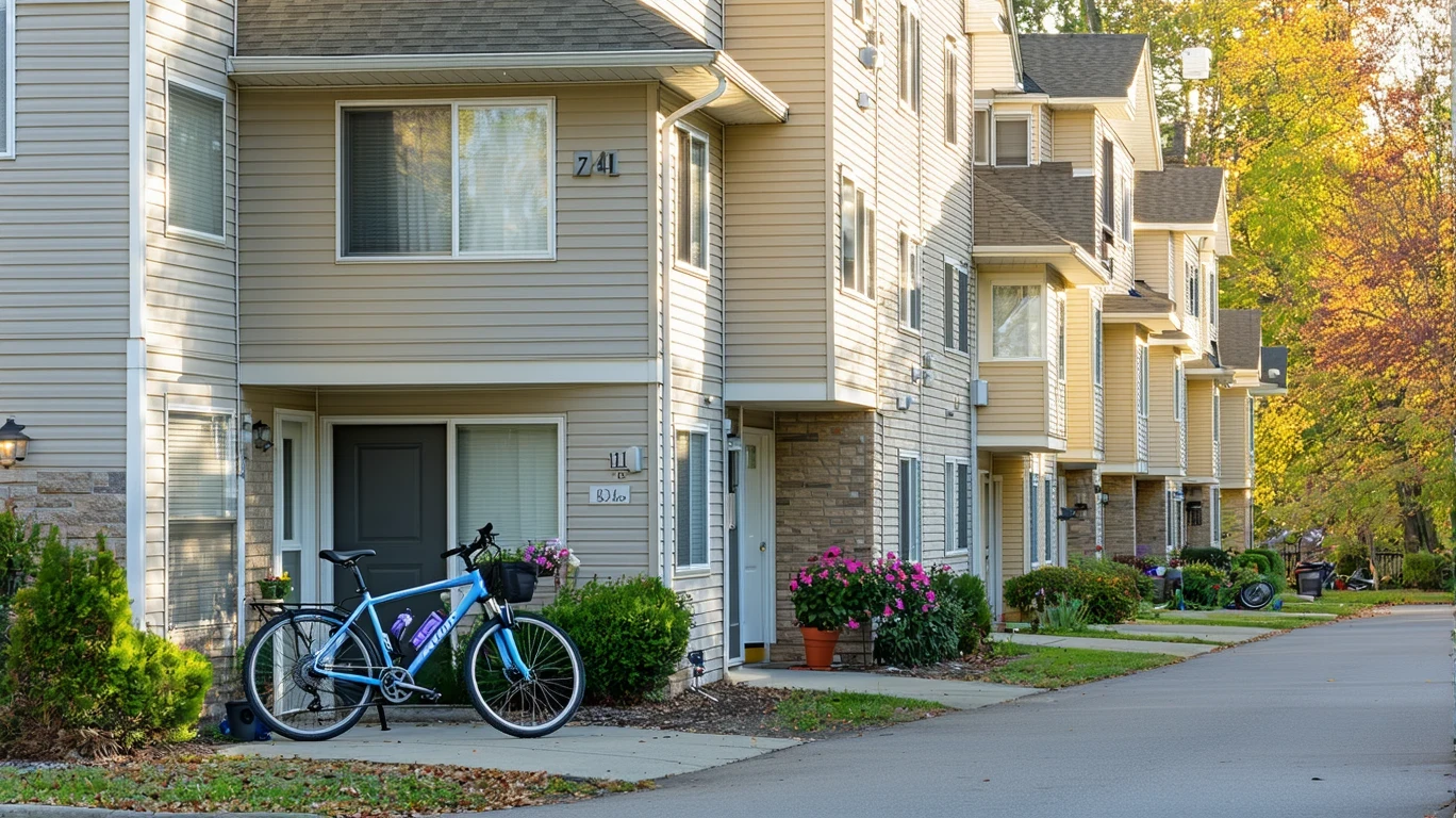
Maple Grove’s housing market centers on single-family homes, with a median home value of $379,800 and median gross rent of $1,768 per month. That entry cost reflects demand for suburban space, newer construction, and access to highly rated school districts. For buyers, the upfront barrier is significant — down payments, closing costs, and ongoing property taxes concentrate financial pressure early. For renters, monthly obligations are predictable but high, and rental stock skews toward larger units rather than studios or one-bedrooms.
Saint Paul’s housing data for 2026 is unavailable, but the city’s structure tells a different story. Mixed building heights, both residential and commercial land use, and rail transit access suggest a broader range of housing types — apartments, duplexes, rowhouses, and older single-family homes. That diversity typically translates to more entry points for renters and first-time buyers, though competition for well-located units near transit can be intense. Without numeric values, we can’t compare prices directly, but we can compare housing form and flexibility: Maple Grove offers space and newer stock at a high entry cost; Saint Paul offers variety and transit proximity with less certainty about availability.
For renters, Maple Grove’s $1,768 median rent reflects larger units and suburban amenities, but limits options for singles or couples seeking smaller, lower-cost apartments. Saint Paul’s mixed housing stock likely provides more flexibility at different price points, especially near transit corridors. For first-time buyers, Maple Grove’s $379,800 median home value sets a clear — and high — entry threshold, while Saint Paul’s older housing stock and varied building types may offer lower entry costs in exchange for older construction and higher maintenance exposure. For families, Maple Grove delivers space and newer homes, but experiential signals show limited family infrastructure (school density below thresholds), meaning parents may face longer drives to schools and activities despite the suburban setting. Saint Paul’s strong family infrastructure — both schools and playgrounds meet density thresholds — reduces logistics friction even if housing stock is older.
Housing takeaway: Maple Grove front-loads cost into entry barriers (high purchase prices, high median rent) but delivers space and newer construction. Saint Paul distributes housing options more broadly across types and price points, with stronger proximity to schools and playgrounds reducing the hidden time cost of family logistics. Households sensitive to entry cost and space may prefer Maple Grove if they can absorb the upfront expense; those prioritizing flexibility, transit access, and lower logistics friction may find Saint Paul’s structure more forgiving, even without numeric confirmation.
Utilities and Energy Costs
Both cities face identical utility rates in 2026: 14.98¢ per kWh for electricity and $9.43 per MCF for natural gas. That shared baseline means differences in utility exposure come from housing stock, home size, and seasonal intensity, not from rate structures. Minnesota’s climate demands serious heating from November through March, with occasional deep freezes driving natural gas usage higher. Summers bring heat and humidity, requiring air conditioning from June through August, though cooling demand is less extreme than heating.
Maple Grove’s housing stock skews newer and larger — single-family homes with modern insulation, efficient HVAC systems, and bigger square footage. Newer construction reduces heating and cooling waste, but larger homes require more energy to maintain comfortable temperatures year-round. A 2,500-square-foot home in Maple Grove will use more electricity and natural gas than a 1,200-square-foot apartment in Saint Paul, even if the Maple Grove home is better insulated. For families in larger homes, winter heating dominates utility bills, with natural gas usage spiking during cold snaps. Summer cooling adds moderate expense, but the primary exposure is seasonal heating volatility.
Saint Paul’s mixed housing stock — older apartments, duplexes, and single-family homes — introduces more variability. Older buildings may have less efficient insulation and aging HVAC systems, increasing both heating and cooling costs per square foot. But smaller units (studios, one-bedrooms, townhouses) require less total energy, offsetting some of the inefficiency. Renters in older buildings face less control over efficiency upgrades, meaning they absorb seasonal volatility without the ability to invest in improvements. Homeowners in older Saint Paul properties can upgrade insulation, windows, and heating systems, but those upgrades require upfront capital and time.
Utility cost exposure varies by household type. Single adults in smaller Saint Paul apartments face lower absolute utility costs due to smaller square footage, but may experience higher per-square-foot costs in older buildings. Couples in Maple Grove’s newer, larger homes benefit from efficiency but pay more in total due to size. families with kids in Maple Grove’s larger homes face the highest absolute utility costs, especially during winter heating months, but gain predictability from newer construction. Families in older Saint Paul homes face moderate costs with higher volatility if insulation and HVAC systems are outdated.
Utility takeaway: Both cities face the same rates, so exposure depends on home size, age, and household heating/cooling habits. Maple Grove’s newer, larger homes deliver predictability but higher total costs due to square footage. Saint Paul’s older, smaller units reduce total costs but introduce volatility, especially for renters in aging buildings. Households prioritizing predictability and efficiency may prefer Maple Grove’s newer stock; those prioritizing lower absolute costs and smaller footprints may find Saint Paul’s smaller units more manageable, even with older infrastructure.
Groceries and Daily Expenses
Grocery costs in both cities reflect the same regional price environment — the RPP index sits at 98 for both Maple Grove and Saint Paul, meaning prices track slightly below the national baseline. Derived estimates for staples show ground beef at $6.60/lb, chicken at $2.01/lb, eggs at $2.45/dozen, and milk at $3.95/half-gallon. Those prices apply across the metro, so differences in grocery pressure come from access, store concentration, and shopping habits, not from price variation.
Maple Grove’s experiential signals show corridor-clustered food and grocery access, meaning stores concentrate along commercial strips rather than spreading evenly across neighborhoods. That structure works well for households with cars and predictable shopping routines — big-box stores, warehouse clubs, and chain grocers offer competitive pricing and wide selection. But it introduces planning friction: running out of milk or needing a last-minute ingredient requires a deliberate trip, not a quick walk. For families managing larger grocery volumes, Maple Grove’s car-dependent, bulk-shopping model reduces per-unit costs but increases time cost and requires storage space.
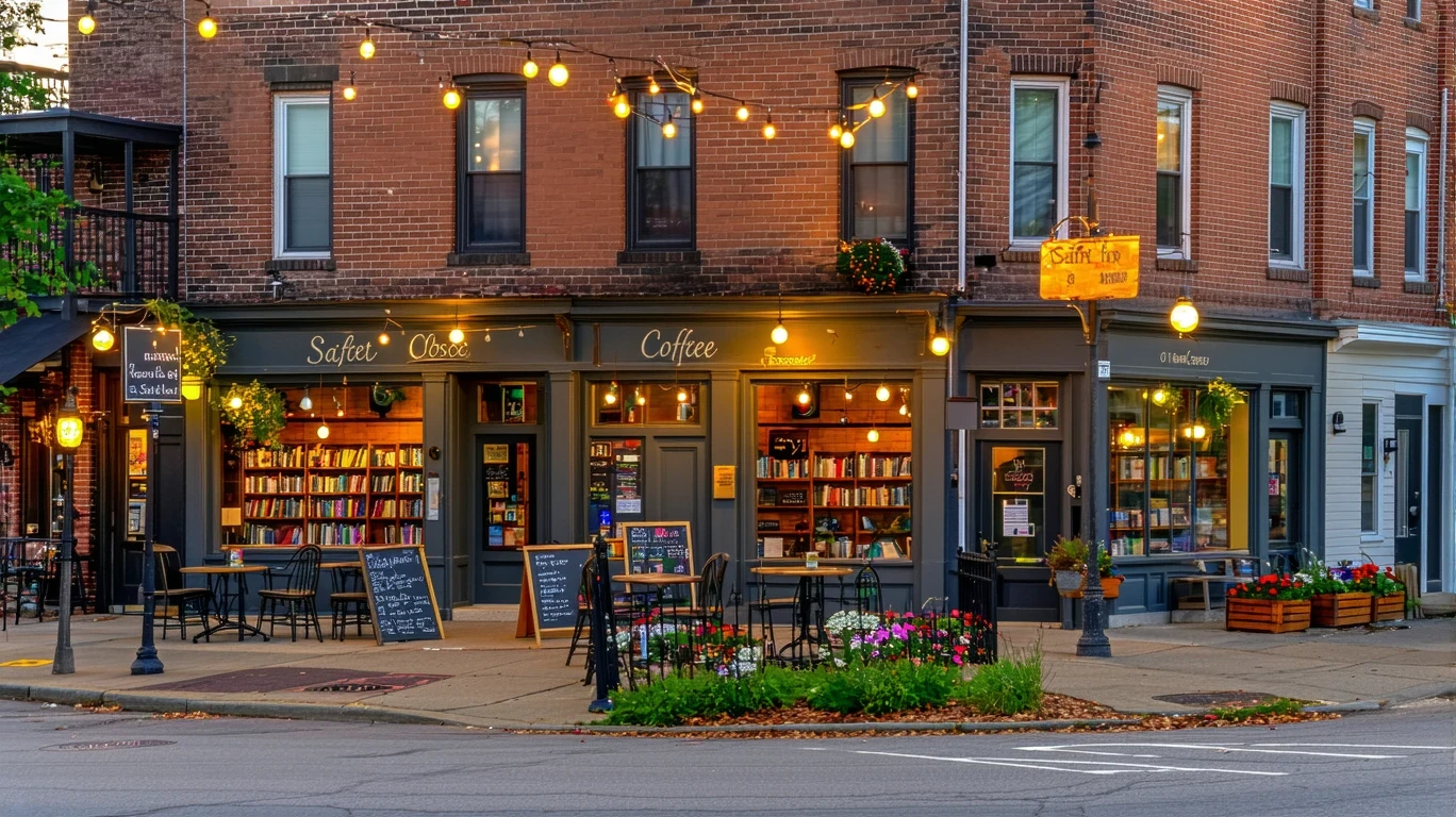
Saint Paul’s experiential signals show broadly accessible food and grocery options, with both food establishments and grocery stores exceeding density thresholds. That structure supports more flexible shopping habits — smaller, more frequent trips to neighborhood stores, corner markets, or co-ops. Prices at smaller stores may run slightly higher than big-box competitors, but the time savings and convenience offset some of that premium. For singles and couples, broadly accessible grocery options reduce the need to plan every trip and allow for walking or transit-based errands. For families, the tradeoff is less clear: smaller stores may not stock bulk items or offer warehouse pricing, pushing larger households back toward car-based shopping even in a more accessible environment.
Daily expenses beyond groceries — coffee, takeout, household goods, personal care — follow similar patterns. Maple Grove’s corridor-clustered structure concentrates chain restaurants, coffee shops, and retail along major roads, making convenience spending car-dependent and trip-bundled. Saint Paul’s broader accessibility spreads convenience options more evenly, making it easier to grab coffee or pick up household items without a dedicated trip. That difference matters more for time-constrained households than for price-sensitive ones: the cost of a latte is the same, but the friction of getting it varies.
Grocery and daily expense takeaway: Prices are nearly identical across both cities, but access structure changes how households shop and spend. Maple Grove fits households with cars, storage space, and time to plan bulk shopping trips — lower per-unit costs, higher time cost. Saint Paul fits households prioritizing flexibility, walkability, and frequent small trips — slightly higher per-unit costs at smaller stores, lower time cost. Families managing large grocery volumes may prefer Maple Grove’s big-box access; singles and couples may find Saint Paul’s broadly accessible options reduce daily friction without meaningful price penalties.
Taxes and Fees
Both Maple Grove and Saint Paul sit in the same state tax environment, meaning Minnesota’s income tax brackets, sales tax rates, and vehicle registration fees apply equally. The primary difference in tax exposure comes from property taxes, which vary by city, school district, and assessed home value. Maple Grove’s median home value of $379,800 sets a clear baseline for property tax calculations, though exact millage rates aren’t provided in the feed. Higher home values typically translate to higher absolute property tax bills, even if rates are comparable, meaning homeowners in Maple Grove face front-loaded, ongoing tax obligations tied to housing entry cost.
Saint Paul’s property tax structure applies to a more varied housing stock — older homes, apartments, duplexes — meaning tax bills vary more widely depending on property type and assessed value. Without numeric housing data for Saint Paul, we can’t compare absolute tax amounts, but the structural difference is clear: Maple Grove concentrates property tax exposure among homeowners in higher-value single-family homes, while Saint Paul distributes it across a broader range of property types and values. Renters in both cities don’t pay property taxes directly, but landlords pass those costs through in rent, meaning renters absorb property tax pressure indirectly without control over assessment or rate changes.
Beyond property taxes, both cities impose local fees for services like trash collection, water, sewer, and stormwater management. Maple Grove’s suburban structure may bundle some services into HOA fees for newer developments, creating predictable monthly obligations but reducing flexibility. Saint Paul’s older, more mixed housing stock typically bills services separately, giving homeowners more visibility into individual costs but introducing more line items to track. Special assessments for street repairs, sidewalk improvements, or utility upgrades can appear in either city, but tend to hit older neighborhoods harder — meaning Saint Paul homeowners may face less predictable one-time fees tied to aging infrastructure.
Tax and fee exposure varies by household type. Homeowners in Maple Grove face higher absolute property taxes due to higher home values, but benefit from newer infrastructure and lower special assessment risk. Homeowners in Saint Paul face more variability — lower property taxes on older, lower-value homes, but higher risk of special assessments and aging infrastructure costs. Renters in both cities absorb property taxes indirectly through rent, but Maple Grove’s higher median rent reflects higher property tax pass-through, while Saint Paul’s varied rental stock creates more price dispersion. Long-term residents in either city benefit from predictable tax structures, but Maple Grove’s newer development and higher home values mean faster assessment growth over time.
Tax and fee takeaway: Maple Grove front-loads tax exposure into higher property taxes tied to higher home values, with more predictable fees and lower special assessment risk. Saint Paul distributes tax exposure across a wider range of property types and values, with more variability and higher risk of one-time infrastructure fees. Homeowners prioritizing predictability and newer infrastructure may prefer Maple Grove’s structure; those prioritizing lower entry costs and tax flexibility may find Saint Paul’s variability more manageable, especially in older, lower-value properties.
Transportation & Commute Reality
Maple Grove’s commute data shows an average commute time of 24 minutes, with 33.7% of workers facing long commutes and only 3.9% working from home. That pattern reflects car-dependent suburban commuting — most workers drive to jobs in Minneapolis, Saint Paul, or other metro employment centers, facing predictable but unavoidable time costs. Experiential signals confirm bus-only transit and notable cycling infrastructure, but the pedestrian-to-road ratio suggests walkability exists in pockets rather than across the entire city. For most households, a car is non-negotiable, and commute time is a fixed cost absorbed daily.
Saint Paul lacks numeric commute data in the feed, but experiential signals show rail transit present, walkable pockets with high pedestrian-to-road ratios, and notable cycling infrastructure. Rail access fundamentally changes commute structure: workers can reach downtown Minneapolis or other metro job centers without driving, reducing fuel costs, parking fees, and vehicle wear. Transit commutes may take longer than driving in ideal conditions, but they eliminate the stress of traffic, parking searches, and weather-related delays. For households near rail stations, car ownership becomes optional rather than mandatory, shifting transportation costs from ongoing fuel and maintenance to occasional rideshare or car rental.
Gas prices sit at $3.44 per gallon in both cities, meaning fuel costs are identical for drivers. But how much you drive differs sharply. Maple Grove’s corridor-clustered errands, limited transit, and suburban job dispersion mean most households drive daily for work, groceries, school drop-offs, and errands. Saint Paul’s rail transit, broadly accessible errands, and mixed land use reduce driving frequency, especially for singles and couples who can walk or bike for daily needs. Families in either city still rely on cars for kid logistics, but Saint Paul’s stronger family infrastructure (schools and playgrounds meeting density thresholds) reduces the distance and frequency of those trips.
Transportation takeaway: Maple Grove requires a car for nearly all households, with 24-minute average commutes and high long-commute exposure creating predictable but unavoidable time and fuel costs. Saint Paul’s rail transit and broadly accessible errands reduce car dependency for singles and couples, shifting transportation costs from daily fuel to occasional transit fares or rideshare. Families in both cities need cars, but Saint Paul’s stronger family infrastructure reduces trip frequency and distance. Households prioritizing suburban space and car-based flexibility fit Maple Grove; those prioritizing transit access and lower car dependency fit Saint Paul.
Cost Structure Comparison
Housing pressure concentrates differently in each city. Maple Grove front-loads cost into high entry barriers — $379,800 median home value, $1,768 median rent — delivering space and newer construction in exchange. Saint Paul distributes housing options more broadly across types and price points, with mixed building heights and varied stock creating more entry flexibility but less certainty about availability. Renters and first-time buyers face higher upfront costs in Maple Grove but gain predictability; those in Saint Paul trade lower entry costs for older stock and more variability. Families in Maple Grove get space but face limited family infrastructure (school density below thresholds), increasing logistics friction despite suburban form. Families in Saint Paul benefit from strong family infrastructure (schools and playgrounds meeting thresholds), reducing trip frequency and time cost even in older housing.
Utilities and energy exposure depend on home size and age, not rates — both cities face 14.98¢/kWh electricity and $9.43/MCF natural gas. Maple Grove’s newer, larger homes deliver efficiency but higher total costs due to square footage, with winter heating dominating seasonal bills. Saint Paul’s older, smaller units reduce total costs but introduce volatility, especially for renters in aging buildings without control over upgrades. Households prioritizing predictability and modern construction fit Maple Grove; those prioritizing lower absolute costs and smaller footprints fit Saint Paul.
Daily living and groceries reflect identical regional pricing (RPP index 98 in both cities), but access structure changes shopping habits and time costs. Maple Grove’s corridor-clustered food and grocery options favor car-based bulk shopping, reducing per-unit costs but requiring planning and storage. Saint Paul’s broadly accessible options support flexible, frequent trips on foot or by transit, with slightly higher per-unit costs at smaller stores offset by time savings. Families managing large grocery volumes may prefer Maple Grove’s big-box access; singles and couples may find Saint Paul’s walkable errands reduce daily friction without meaningful price penalties.
Transportation and access create the sharpest structural difference. Maple Grove requires a car for nearly all households, with 24-minute average commutes, 33.7% long-commute exposure, and bus-only transit limiting alternatives. Saint Paul’s rail transit, walkable errands, and broadly accessible daily needs reduce car dependency for singles and couples, shifting costs from daily fuel to occasional transit fares. Families in both cities need cars, but Saint Paul’s stronger family infrastructure reduces trip frequency and distance, lowering time cost even when driving remains necessary.
Decision framing: The better choice depends on which costs dominate your household and which tradeoffs you can absorb. Households sensitive to entry cost and ongoing car expenses may find Saint Paul’s transit access and lower housing entry barriers more forgiving. Households prioritizing space, newer construction, and car-based flexibility may prefer Maple Grove’s suburban structure despite higher upfront and ongoing costs. For families, the difference is less about price and more about logistics friction: Maple Grove offers space but limited family infrastructure; Saint Paul offers strong family infrastructure but older housing stock. For singles and couples, the difference is less about total cost and more about time vs. money: Maple Grove requires a car and planning; Saint Paul offers transit and walkable convenience.
How the Same Income Feels in Maple Grove vs Saint Paul
Single Adult
In Maple Grove, housing and transportation become non-negotiable first — rent skews toward larger units, and a car is essential for work and errands. Flexibility exists in dining and entertainment, but daily logistics require planning and time. In Saint Paul, rail transit and broadly accessible errands reduce car dependency, shifting budget pressure from transportation to housing choice. Flexibility exists in housing type and commute method, with walkable neighborhoods offering more control over time cost than cash cost.
Dual-Income Couple
In Maple Grove, housing entry costs absorb a larger share of combined income, but space and newer construction deliver predictability in utilities and maintenance. Transportation requires two cars if both partners commute, concentrating ongoing costs in fuel, insurance, and parking. In Saint Paul, rail transit allows one-car or no-car households, reducing transportation costs but requiring proximity to transit for maximum benefit. Housing flexibility increases with varied stock, but older construction introduces maintenance and utility volatility that newer Maple Grove homes avoid.
Family with Kids
In Maple Grove, housing costs front-load into high purchase prices or rent, but space accommodates growing families and newer construction reduces maintenance surprises. Limited family infrastructure means longer drives to schools and activities, increasing time cost and fuel expenses despite suburban proximity. In Saint Paul, strong family infrastructure reduces logistics friction — schools and playgrounds meet density thresholds, shortening trip distances and frequency. Older housing stock requires more maintenance and introduces utility volatility, but lower entry costs and transit access free up budget flexibility for childcare or activities.
Decision Matrix: Which City Fits Which Household?
| Decision factor | If you’re sensitive to this… | Maple Grove tends to fit when… | Saint Paul tends to fit when… |
|---|---|---|---|
| Housing entry + space needs | You need predictable housing costs and modern construction | You can absorb high upfront costs for space and newer stock | You prioritize entry flexibility and varied housing types over newness |
| Transportation dependence + commute friction | You want to minimize car dependency and fuel costs | You prefer car-based flexibility and can absorb daily driving time | You value rail transit access and walkable errands over driving convenience |
| Utility variability + home size exposure | You want predictable utility bills and efficient heating/cooling | You prioritize newer construction and can absorb higher total costs from larger homes | You prefer smaller footprints and lower absolute costs despite older infrastructure |
| Grocery strategy + convenience spending creep | You want to control per-unit costs through bulk shopping | You have storage space and time to plan corridor-based shopping trips | You value walkable access and frequent small trips over bulk pricing |
| Fees + friction costs (HOA, services, upkeep) | You want predictable monthly fees and lower special assessment risk | You prefer bundled services and newer infrastructure despite higher property taxes | You can manage variability and one-time fees in exchange for lower baseline costs |
| Time budget (schedule flexibility, errands, logistics) | You want to minimize daily logistics friction and trip planning | You can absorb time costs from car-dependent errands and longer kid logistics | You prioritize walkable errands and strong family infrastructure reducing trip frequency |
Lifestyle Fit
Maple Grove delivers suburban space, newer housing stock, and access to parks and green space — experiential signals show park density exceeding high thresholds, with water features adding outdoor appeal. The city’s mixed building heights and residential-commercial land use create pockets of walkability, and notable cycling infrastructure supports recreational biking. But daily life requires a car: errands cluster along commercial corridors, transit is bus-only, and the 24-minute average commute reflects car-dependent job access. For households prioritizing space, outdoor access, and modern construction, Maple Grove fits well — as long as driving and trip planning don’t feel burdensome.
Saint Paul offers rail transit, broadly accessible errands, and strong family infrastructure, creating a lifestyle centered on walkability, transit access, and reduced logistics friction. Experiential signals show high pedestrian-to-road ratios, rail stations, and both food and grocery density exceeding thresholds. Park density is high, with water features present, and both schools and playgrounds meet density thresholds, making family logistics easier despite older housing stock. Mixed building heights and residential-commercial land use support neighborhood-based living, where daily needs are within walking or biking distance. For households prioritizing transit access, walkable convenience, and lower car dependency, Saint Paul fits well — even if housing stock is older and maintenance costs are less predictable.
Lifestyle factors indirectly affect costs in both cities. Maple Grove’s car dependence increases transportation expenses but reduces time spent navigating transit schedules or walking in harsh winter weather. Saint Paul’s rail access and walkable errands reduce fuel costs but require proximity to transit for maximum benefit, and winter walking can be challenging during deep freezes. Maple Grove’s newer housing stock lowers maintenance and utility volatility, while Saint Paul’s older stock increases both but offers more housing type flexibility. Outdoor access is strong in both cities, with high park density and water features supporting recreation without additional cost. Family infrastructure differs sharply: Saint Paul’s strong school and playground density reduces logistics friction, while Maple Grove’s limited family infrastructure (school density below thresholds) increases trip frequency and distance despite suburban form.
Quick facts: Maple Grove’s unemployment rate sits at 2.8%, reflecting a strong local job market, while Saint Paul’s 2.9% unemployment rate is nearly identical, showing comparable economic stability across both cities. Both cities share the same RPP index of 98, meaning regional prices track slightly below the national baseline, with no meaningful cost-of-living difference driven by price levels alone.
Frequently Asked Questions
Is Maple Grove or Saint Paul cheaper for families in 2026?
Neither city is universally cheaper — the better fit depends on which costs dominate your household. Maple Grove front-loads cost into housing entry ($379,800 median home value, $1,768 median rent) but delivers space and newer construction. Saint Paul offers more housing type flexibility and strong family infrastructure (schools and playgrounds meeting density thresholds), reducing logistics friction despite older stock. Families sensitive to entry cost and trip frequency may prefer Saint Paul; those prioritizing space and modern construction may prefer Maple Grove.
Can you live in Saint Paul without a car in 2026?
Yes, especially for singles and couples near rail transit. Saint Paul’s rail service, broadly accessible errands, and high pedestrian-to-road ratios support car-free or one-car households. Families still need cars for kid logistics, but strong family infrastructure (schools and playgrounds meeting thresholds) reduces trip distance and frequency compared to Maple Grove, where limited family infrastructure increases driving despite suburban form